Feidad 2006 | Guillem Baraut | Mattia Gambardella

04
Process

Slender multistress driven structures
Guillem Baraut
Mattia Gambardella

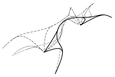
FINAL DESIGN STRATEGY

Once revised and analysed all the experiments carried out in both physical and digital realms, a final design strategy is developed.

Just the most successful physical experiments and digital tools will be used for that purpose. In this case the wool threads and the catenaries experiments are the ones that are chosen in order to inform the digital tools, that are the topology optimization code in Matlab, the minimizing paths system algorithm in Generative components, and the Finite Elements Analysis software Ansys for both structural analysis and 3D topology optimization.

In the local scale the experiments chosen are the foam as a form for laying out the fibers, and the lycra knot to study how to lay out fibers in complex geometries.

In the last stage the manufacturing techniques that are considered are the racing boats sails, for the laying out of fibers just where they are needed, the CNC cut foam that will be the form where the fibers will be laid out, and the casting of the biggest pieces possible in a factory and special transportation to the site. For the microscale we choose using single fibers or textile fibers with a main direction, but not the pultrusion techniques.

PROCESS SET UP

This design methodology combines structural topology optimization in a routine in Matlab with a minimizing path system algorithm implemented in Generative Components. The first script in Matlab is, in the first go, informed by the wool threads physical experiment in terms of initial branches and position of the branching points. The first run the routine is providing the first spatial configuration.

A pedestrian bridge is developed in order to explain how this methodology works. This bridge will respond to the following variables:
- Number of access to the bridge
- Accesses spatial position
- Flow dimension

The program tend to optimize the distribution of the stiffness in such a way to redistribute evenly the stresses. The use of the Mathlab routine as a mapping tool provides new potentialities within the design process.

When having the first results from the topology optimization they are mapped as a vector field in GC in order to provide the initial configuration for the minimum road algorithm. This vector field is mapped on a 3D surface defined according to the catenaries physical experiments and the first topology optimization in elevation in 2D.

Those mapped points from the topology optimization will represent the digital areas in which run the path length optimization algorithm.

A spline tracing algorithm is run amongst those points: in several iterations the starting and ending points of each side are connected between them by a family of curves.

Amongst those lines (potential minimum path) just a few are picked by the computer as the shortest solution to that specific connection problem.

Once the Path is optimized through the script, the points composing its shape are exported again into Matlab to run for the second time the topology optimzation script.

This process can be run automatically several times until the designer found that the requirements are successfully achieved.

The figure 1 on the left show the initial topology optimizations in plan and elevation for a bridge that is linking 3 and 3 points. This information is then mapped into a Generative Components parametric model. The first images in figure 2 show how some repellors and attractors informed by the catenaries physical experiments define a 3D surface. The results from Matlab are mapped on this surface, and then the minimizing path algorithm start running.

The shorter paths from the last image of figure 2 are then imported again into Matlab (figure 3) in order to run again the topology optimization algorithm, affected by this new information.

The process continue until the user consider that a successful solution is achieved. In Figure 4 there are the final steps of the methodology consisting in getting the shortest paths of the minimizing algorithm, and running another script that defines the material distribution on this structure.

DESIGN PROCESS

The design process is defined by a digital tool that is working following this scheme:

i. Start with topology optimization in Matlab that is informed by physical experiments (wool threads).

ii. Export structure 2D and map a 3D surface created in GC.
This surface is developed according to the results of the catenaries experiments. Run the minimal path algorithm and export the results to Matlab.

iii. & iv. Run the topology optimization and minimal path in GC iteratively until finding the result that the user is looking for.

v. On the final geometry we develop a parametric model that maps the material on the paths according to the stress vector field of the optimized structure.

It is interesting to highlight that there exists a crossed relation between the physical experiments and digital tools that are related to minimal path and structural performance.

In that sense the topology optimization code, a structural performance based software, is informed from the beginning by the wool threads experiments, that are directly related to minimal path.

The same happens with the Generative Components models, that basically consist in a minimizing path algorithm that is informed by the catenaries physical experiments, directly related to structural performance.

STRESS VECTOR FIELD

The direction of principal stress is the one for which there is no shear stress. The two or three principal stresses (in a surface or in a volume) are always perpendicular. With this consideration the fiber material can be placed with the direction of the stresses. In that case the material can be working at 100% of its capacity, because it will not be any redundant material in any direction.

From this study we conclude that the best solution for the definition of the final design is to drive the position and direction of the material according to the principal stresses vector field.

This vector field will be defined through a process of optimization in 3D with Ansys.

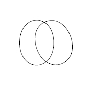
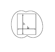
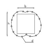
In Figure 3 there is the same two dimensional example of the single span beam with the main direction of the stresses highlighted in red.

The figure shows how the angle a is varying from 45º when the shear is maximum and with a low bending moment, to around 30º at the left side when there is maximum negative bending moment and maximum shear. At the centre of the beam, with no shear and with maximum bending moment the angle turns to 0º.

These results are almost the same that were defined by the topology optimization carried out previously, and that can be seen at the tables of the previous pages.

TRANSLATION FROM VECTOR FIELD TO GC

The Finite Elements Analysis method can take a long time for a big structure, and the process of transferring the vector field data to Generative Components can be even slower.

In order to avoid that, the way the fibers are defined in Generative Components is according to the vector field principles, but without calculating it for every single piece of the structure.

The way for doing that is translating the angle a from the vector field to every position along the structure.

The angle can vary depending on the distance to the supports, or the position along the structure. For that reason the way we define the angle is according to the T value along the curve of the path, that has been defined trough the Macroscale process.

In Generative Components the process to do that is:
- Generate some points on the curve according to the T value
- The distance or spacing from one point to the other is directly related to the angle of the vector field
- Generate splines around the ellipses with a regular pattern of crossings. According to the distance between the ellipses these crosses will occur with a more pronounced angle, or they will be almost horizontal. The longer the spacing is, the more horizontal the splines will be.

At the end, the pattern of the splines crossing around the ellipses is according to the stress vector field.

The dimensions of the ellipses are defined according to manufacturing and spatial requirements.

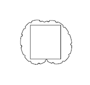
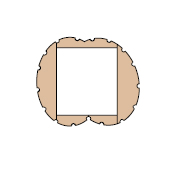
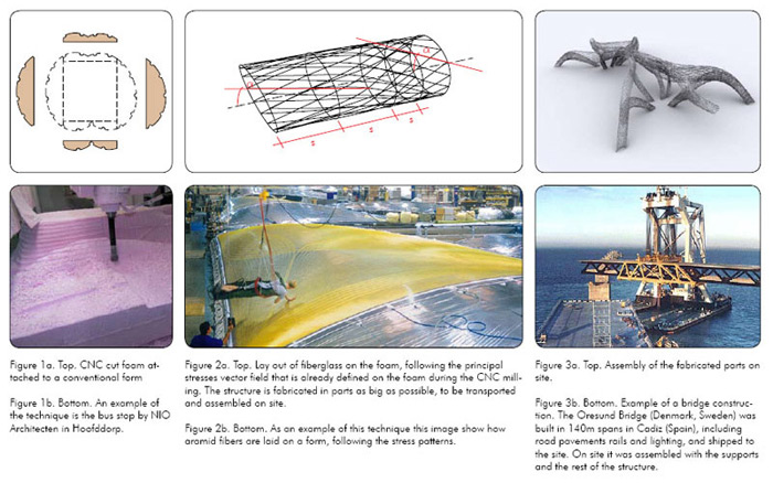
MANUFACTURING PROCESS

In order to summarize the manufacturing process figures 1 to 3 shows the main steps.

The methodology explained defines the 3D model until the CNC pieces to be cut. These pieces are then sent to manufacturing as figure 1 shows.

After being cut the foam pieces are assembled together in a factory on a conventional form and scaffolding.

On these pieces the glass fibers are laid out with resin. The fibers follows the traces that the CNC milling machine drew on the foam.
These traces are digitally defined according to the principal stresses vector field. Figure 2 shows this process with a real example, the manufacturing of sails for racing boats.

On the factory the structure is built in pieces as big as they are able to transport on site. These pieces are then shipped on site and assembled together. The limits of this technique are even more than hundred metres, as can be seen in figure 3 with the Oresund bridge example.